Chem Copilot User Guide: Tabular Formulation Modeling & In-Silico Experimentation

Chem Copilot’s Lab Assistant provides a self-service, no-code environment designed to transform physical laboratory formulation data into predictive intelligence.

Unlike small-molecule discovery tools that require 2D/3D chemical structures or molecular embeddings, the Formulation Modeling Module learns directly from tabular mixture proportions and process variables (such as ingredient weights, volume ratios, processing temperatures, or curing times).

This guide details how to navigate the platform, configure formulation models, run in-silico parameter sweeps, analyze design spaces, and execute iterative R&D cycles.

In this demonstration, we use a concrete formulation dataset containing experimental history, mixture variables, curing conditions, and measured compressive strength to build and evaluate a machine learning model.

Step 1: Data Preparation & Column Formatting

To model physical mixtures, navigate to the Programs page and select the formulation workspace.

[ Tabular Dataset (CSV/Excel) ] ──> [ Select Mixture Inputs ] ──> [ Assign Performance Target ]

Dataset Structure Requirements

• Rows & Columns: Each row represents a unique physical formulation alongside its measured laboratory test results.

• Variable Types: Input columns can be numeric or categorical in nature (e.g., ingredient quantities, supplier types, process conditions).

• No Chemical Embeddings Needed: Because the algorithms train directly on tabular mixture columns, no chemical embedding preprocessing is required.

⚠️ Critical Rule for Codependent Variables: Select only one set of codependent variables during model setup. For example, include ingredient amounts in kilograms or weight percentages, but never both. Including redundant representations distorts tabular variable training.

Step 2: Model Setup, Training & Diagnostic Evaluation

Once your data is loaded, configure and train your formulation model by selecting your preferred model architectures, choosing your input columns, and assigning your performance target (e.g., compressive strength, viscosity, tensile durability, or release rate).

Evaluating Accuracy Metrics

Model performance is evaluated via prediction-versus-actual correlation graphs generated through five-fold cross-validation:

• R-Squared ($R^2$): Measures correlation strength and overall fit quality.

• Root-Mean-Square Error (RMSE): Quantifies absolute prediction error margins in physical measurement units.

Interpreting Feature Influence

Because inputs represent recognizable physical quantities (e.g., primary binder amount, water ratio, or aging duration), feature influence scoring is easy to interpret. The top-ranked variables highlight the primary drivers of performance, signaling exactly where future experimentation should focus.

Step 3: Running In-Silico Parameter Sweeps (Sensitivity Analysis)

Parameter sweeping enables you to perform in-silico sensitivity analyses. By varying inputs systematically, the model generates component ladders and trend analyses before you mix a single physical batch in the lab.

[ Select Baseline Formulation ] ──> [ Define Sweep & Fixed Ranges ] ──> [ Generate Combinatorial Grid ]

How to Configure a Sweep:

1. Choose a Baseline: Select an existing physical formulation to serve as your starting point.

2. Assign Variable Rules: Specify which variables remain fixed and which variables will sweep.

3. Set Sample Increments: Choose the number of sweep samples to evaluate across each variable's range.

Extrapolation Warnings

The system automatically displays the observed range from your training dataset. If a chosen sweep range attempts to extrapolate too far beyond historical bounds, the platform issues a warning, as predictions outside recommended bounds carry increased uncertainty.

Combinatorial Candidate Generation

The platform automatically calculates the total number of virtual experiments generated by multiplying the selected sample increments:

$$\text{Total Virtual Formulations} = \text{Samples}_{\text{Var A}} \times \text{Samples}_{\text{Var B}}$$

(For example, sweeping 15 values of Variable A across 10 values of Variable B generates 150 candidate formulations instantly).

The model scores all generated sweep rows in real time, allowing you to identify high-performing design spaces while adhering to practical formulation constraints.

Step 4: Visualizing Design Space & Selecting Candidates

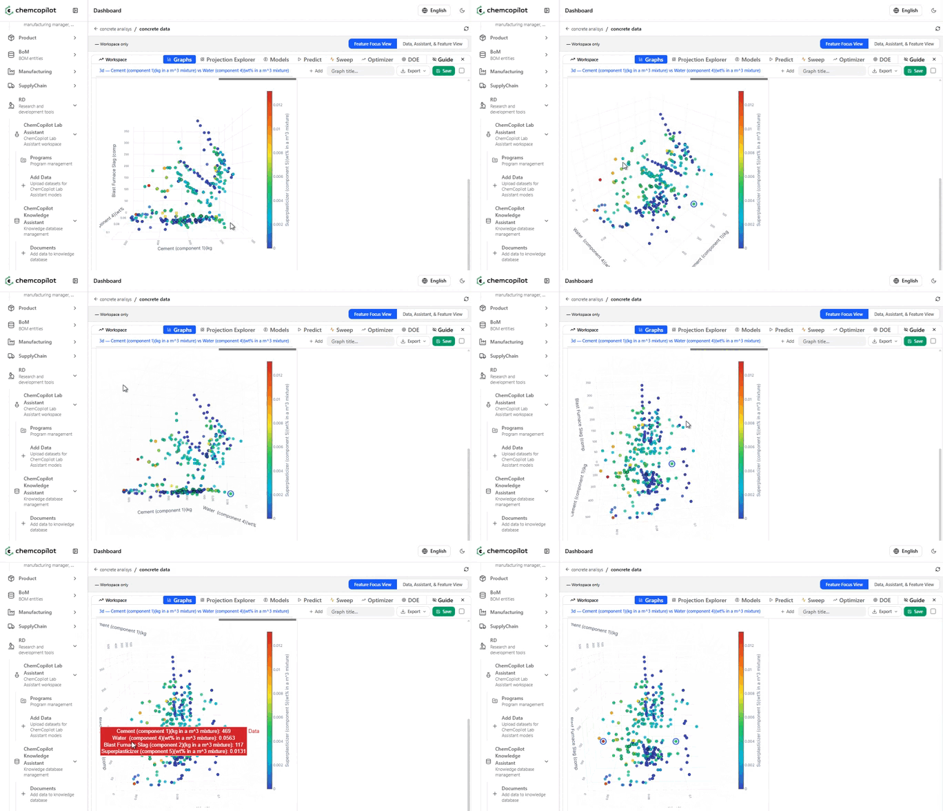
To evaluate virtual predictions alongside physical bench measurements, formulations are projected into a dimensionally reduced visual design space.

Visual ElementMeaning & Actionable InsightProximity

Indicates overall formulation and process condition similarity.

Clusters

Show regions of consistent, predictable formulation behavior.

Sparse Regions

Highlight gaps in your historical data where new experiments can improve overall model coverage.

Heatmap Overlays

Reveal performance hot-spots across selected mixture and process variables.

Response Surfaces

Zooming into sweep data displays multi-variable response surfaces for precise candidate selection.

Exporting Candidates

Selecting preferred virtual formulations adds their information cards to the Favorites Area. From there, you can perform detailed formulation comparisons and export digital recipes directly for laboratory execution.

Step 5: The Iterative Closed-Loop R&D Workflow

Chem Copilot is designed to support a continuous, self-reinforcing discovery loop:

┌────────────────────────────────────────────────────────────────────────┐
│                   THE CLOSED-LOOP DISCOVERY CYCLE                      │
│                                                                        │
│   1. Select Virtual Candidates  ──>  2. Conduct Physical Lab Tests     │
│           ▲                                      │                     │
│           │                                      ▼                     │
│   4. Generate Refined Sweeps   <──  3. Append Data & Retrain Model     │
└────────────────────────────────────────────────────────────────────────┘

1. Physical Validation: Mix and test your top-selected virtual candidates in the physical laboratory.

2. Data Integration: Append the newly measured test results to your original training dataset.

3. Model Retraining: Retrain your model on the expanded dataset.

4. Target Refinement: Use the improved, higher-coverage model to hone in on your exact performance targets.

Security & Cloud Architecture

Chem Copilot operates as a self-service, no-code, secure cloud environment. The platform connects data, surrogate models, virtual predictions, and next-experiment recommendations while maintaining strict privacy boundaries—your proprietary laboratory data is never shared with other users or outside models.