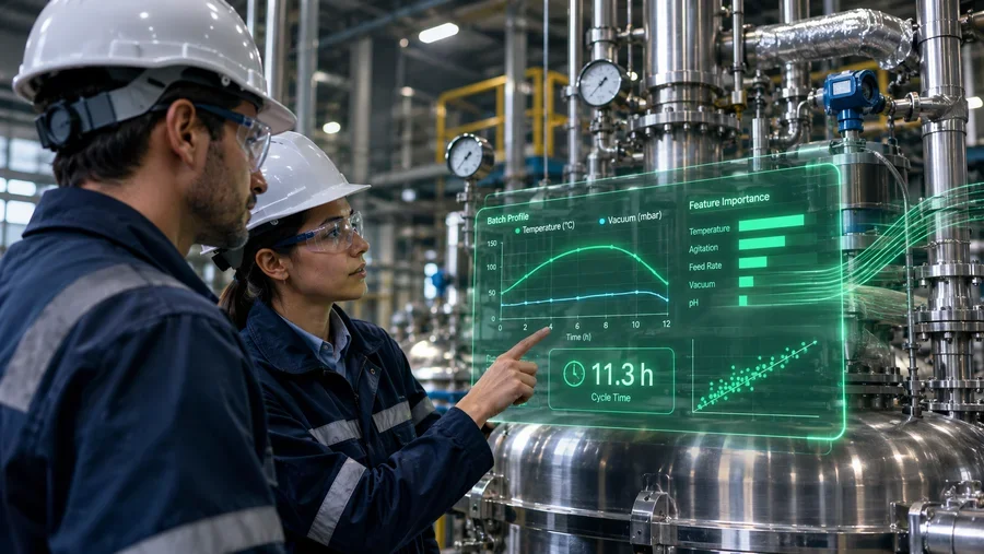
Most batch recipes were tuned once, years ago, by an engineer who no longer works at the plant. The heating ramp, the hold temperature, the vacuum profile, the agitator speed: each was set conservatively, then locked by a change-control process that makes revisiting them feel riskier than leaving money on the table. If you run a batch reactor at or near capacity, every hour of cycle time is throughput you cannot sell. Chemical process optimization AI exists to reopen that recipe without reopening the risk. This article walks through an anonymized case: a specialty polyester resin team that used historian data from 214 historical batches, a surrogate model, and constrained Bayesian optimization to take a 14.5-hour cycle down to 11.3 hours, with no capital spend and no new 48-run DOE.
The Starting Point: 214 Batches, 9 Tags, and a 14.5-Hour Cycle
The process was a two-stage esterification run in a 12 m³ jacketed glass-lined reactor. Stage one heated the charge to reaction temperature under nitrogen; stage two pulled vacuum to drive off water of condensation until acid value hit the release spec. The nominal recipe called for a 14.5-hour cycle, but the historian told a messier story: real cycles ranged from 12.9 to 17.8 hours, and nobody could say with confidence why.
The team had nine tags they trusted. Jacket inlet temperature, batch temperature, vacuum level, agitator speed, nitrogen sparge rate, catalyst charge, raw material lot acid value, ambient cooling-water temperature, and the acid value at each in-process sample. They also had something most teams underestimate: 214 completed batches of the same grade, logged over 31 months, with release results attached in the LIMS.
That dataset was never collected for modeling. It was collected for compliance and traceability. But 214 batches with consistent tags is more than enough to train a reliable surrogate model, provided the data is structured correctly before anyone touches an algorithm.
Step 1: Structuring Historian Data for Chemical Process Optimization AI
The first three weeks of the project produced no model at all. They produced a clean table. Historian exports arrive as time series at irregular intervals, with different tags sampled at different rates, alarm gaps, and recipe steps that are not labeled in the data stream. Batch 087 might have a 40-minute hold because of a utility interruption, not because of a recipe decision. Feeding that directly into a regression model teaches the model that random downtime is a process variable.
The process engineer and a data analyst built a batch-level feature table. Each row was one batch; each column was a summarized recipe decision or input condition, not a raw sensor trace. Heating ramp rate became a single number (°C/min between 60 °C and reaction temperature). Vacuum profile became three numbers: time to reach 50 mbar, minimum pressure held, and duration at minimum. Raw material variation entered as the incoming lot acid value and hydroxyl number. Utility disruptions were flagged and the 11 affected batches were excluded from training rather than left in to distort it.
The target variable was total cycle time to acid value release, but the team added two secondary targets they were not willing to trade away: final color (Gardner) and molecular weight dispersity, both of which had historically drifted when operators pushed temperature.
Twenty-three features, three targets, 203 usable batches. That is a small dataset by consumer-tech standards and a large one by chemical process standards. Tree-based models handle it well; neural networks generally do not at this scale.
Step 2: Finding What Actually Drove Cycle Time
Before optimizing anything, the team wanted to know which variables mattered. A gradient boosting model trained on the 203 batches reached a cross-validated R² of 0.81 for cycle time, which was good enough to trust directionally but not good enough to trust blindly, a distinction that shaped everything that followed.
Feature importance and SHAP values told a story the team half-expected and half-did not. The two largest contributors were the time to reach 50 mbar in stage two and the incoming lot acid value. The first was a recipe decision the operators controlled; the second was a raw material property nobody had been compensating for. Batches that received a high-acid-value lot were running 1.5 to 2 hours longer, and operators had been treating that as normal variability rather than something the recipe could respond to.
Agitator speed, long assumed to be a lever, ranked seventh. Within the range the plant had actually run (60 to 85 rpm), it had almost no measurable effect on cycle time. That finding alone saved the team from spending confirmation batches on a variable that did not matter.
This is the same diagnostic logic described in our guide to finding the root cause of batch variability with machine learning: the model is used first as an interrogation tool, and only afterward as an optimization engine. Teams that skip the interrogation step tend to optimize the wrong knobs.
Step 3: Bayesian Optimization Inside Hard Safety Constraints
With the drivers understood, the team moved to optimization. The question was not "what is the fastest possible recipe" but "what is the fastest recipe that stays inside the operating envelope, holds color below Gardner 3, keeps dispersity in spec, and never exceeds the jacket's 185 °C limit."
Bayesian optimization was chosen over a classical response-surface DOE for two reasons. First, it could start from the 203 historical batches instead of requiring a fresh designed run set. Second, it proposes one batch at a time and updates after each result, which fit a plant that could spare one confirmation batch per week but not twelve in a row. The trade-offs between these two approaches are covered in RSM vs Bayesian optimization for chemical process DOE; the short version is that Bayesian optimization wins when you already have data and want to spend as few new runs as possible.
The comparison below shows the options the team weighed and why they landed where they did.
| Approach | New batches needed | Uses historian data | Handles constraints | Verdict for this case |
|---|---|---|---|---|
| Operator experience / recipe tweaks | Unbounded | Informally | By instinct | Status quo; produced the 12.9–17.8 h spread |
| One-factor-at-a-time trials | 20–30 | No | Poorly; misses interactions | Too slow, blind to interactions |
| Classical RSM (central composite) | ~30 for 4 factors | No | Yes, via desirability | Rigorous but ignores 203 existing batches |
| Surrogate model + Bayesian optimization | 8–12 sequential | Yes, as the prior | Yes, as hard bounds | Selected |
| Reinforcement learning controller | Hundreds of episodes | Partly, for simulation | Requires reward shaping | Overkill for a fixed-recipe batch |
Three guardrails were non-negotiable. Every proposed recipe had to fall inside the range of conditions the plant had already run, with a 10% margin, because the surrogate model has no idea what happens outside the data it was trained on. Every proposal had to be reviewed and signed off by the process engineer before it reached the control room. And the acquisition function was configured to penalize predictions with high uncertainty, so the optimizer leaned toward confident improvements rather than speculative leaps.
Results After 12 Confirmation Batches
The optimizer's first three proposals were modest: a steeper vacuum pull-down in stage two and a catalyst charge adjusted by lot acid value. Cycle time dropped to 13.1 hours on the first confirmation batch and 12.6 on the third. Proposals four through eight explored a slightly higher stage-one hold temperature combined with the faster vacuum profile; two of those batches showed color creeping toward the Gardner 3 limit, and the model learned to back off. By batch twelve the recipe had stabilized.
| Metric | Baseline (203 batches) | Optimized (last 6 confirmation batches) |
|---|---|---|
| Mean cycle time | 14.5 h | 11.3 h (−22%) |
| Cycle time range | 12.9–17.8 h | 10.9–11.8 h |
| Color (Gardner) | 2.1 avg, max 3.4 | 2.3 avg, max 2.8 |
| Dispersity out-of-spec | 4 of 203 | 0 of 12 |
| Confirmation batches used | — | 12 over 11 weeks |
Two things in that table matter more than the headline 22%. The cycle time range collapsed from nearly five hours to under one, which is what scheduling actually needs. And color variability went down, not up, because the lot-aware catalyst charge removed a source of inconsistency that had been there all along. Faster and more consistent are usually presented as a trade-off; here they came from the same change.
On a reactor running roughly 180 batches per year, 3.2 hours per batch is about 24 additional days of reactor availability annually, which the plant converted into a second grade it had previously been outsourcing.
What Made It Work, and What Would Have Broken It
The honest summary is that the algorithm was the easy part. Gradient boosting and Bayesian optimization are mature, and the configuration took an afternoon. The hard parts were upstream and downstream of the model.
Upstream, the batch-level feature table was the single most important artifact in the project. Teams that try to optimize directly on raw time-series tags without summarizing them into recipe decisions usually get a model that predicts well in cross-validation and proposes nonsense in the plant. Downstream, the process engineer's veto on every proposal was not a formality. Proposal six would have exceeded the jacket limit under a plausible fouling scenario the model had never seen, and it was rejected before it ran.
This workflow, historian ingestion, feature engineering, no-code surrogate modeling with gradient boosting, and constrained Bayesian optimization with an engineer in the loop, is the pattern ChemCopilot's process optimization and Digital Twin features were built around, including the SAP and historian connectors that move the data in without a custom integration project. But the pattern is the point, not the tool. A team with Python and patience can replicate it; a team without the feature table and the engineering veto cannot, regardless of platform.
Three conditions would have sunk the project. Fewer than roughly 60 to 80 consistent batches, below which the surrogate model's uncertainty is too wide to guide anything. Historian tags that had been renamed or recalibrated mid-dataset without a record. And a release spec that was itself inconsistent across the period, which would have made the target variable meaningless. Check for all three before committing a single engineering hour.
Key Takeaways
Historian data collected for compliance is usually sufficient to train a surrogate model for chemical process optimization AI, provided it is restructured into a batch-level feature table and utility disruptions are excluded. Use the model first to identify which variables actually drive the outcome; in this case, a raw material property nobody was compensating for ranked second. Bayesian optimization with hard constraints and an engineer approving every proposal spent 12 batches where a fresh RSM would have spent 30, and delivered a tighter distribution, not just a faster mean.
FAQ
How much historian data do you need for chemical process optimization AI?
For a fixed-recipe batch process with 15 to 25 summarized features, somewhere between 60 and 100 consistent batches is a practical floor for a tree-based surrogate model. Below that, the model's uncertainty is too wide to guide optimization safely. More batches help, but consistency of tags, recipe steps, and release methods matters more than count.
Why use Bayesian optimization instead of a classical DOE on an existing process?
Classical DOE assumes you are starting from nothing and designs a run set to map the response surface efficiently. Bayesian optimization can treat your historical batches as the prior, so it skips the mapping phase and proposes one improvement at a time. When the plant can spare one confirmation batch per week rather than a block of thirty, the sequential approach fits the operating reality.
Can this approach change the recipe outside the historical operating range?
It should not, and the case above deliberately bounded proposals to the range already run plus a small margin. A surrogate model trained on historian data has no physical knowledge of what happens beyond that range. Extrapolating is where first-principles models or a carefully designed exploratory DOE belong, with appropriate safety review.
Does the process engineer still need to approve every proposed batch?
Yes. The model does not know about fouling history, upcoming maintenance, or a lot of raw material that looks fine on paper but came from a new supplier. In this case one of twelve proposals was rejected on engineering judgment, and that rejection prevented a jacket overtemperature. The engineer-in-the-loop step is a feature of the method, not a limitation.
If your batch reactors are running on recipes nobody has revisited in years, and your historian has a few hundred batches sitting in it, the raw material for this kind of project is already there. Talk to our team about chemical process optimization and we will walk through what your data would support.