Time-Series AI for Chemical Process Monitoring: Plant Engineer’s Guide

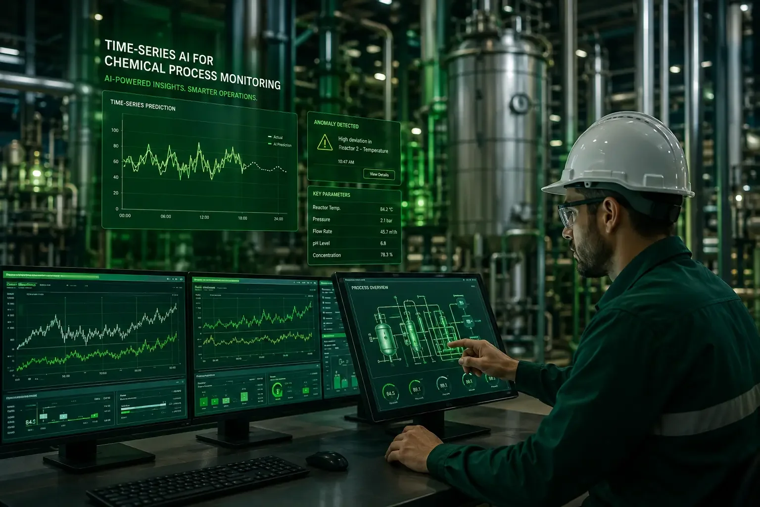
Modern chemical manufacturing plants generate millions of telemetry data points every minute across continuous and batch unit operations. Distributed Control Systems (DCS) and Supervisory Control and Data Acquisition (SCADA) platforms collect temperature, pressure, flow, level, and analytical streams, but traditionally rely on static, single-variable alarm thresholds. This legacy approach results in severe alarm floods during process upsets, unmodeled multivariate failures, and missed opportunities for predictive control.

Time-series artificial intelligence (AI) fundamentally transforms chemical process monitoring. By modeling continuous multivariate sensor streams as dynamic temporal sequences, time-series AI detects subtle operational drift hours before static thresholds trip, predicts off-spec product quality using virtual inferential sensors (soft sensors), and prevents catastrophic events such as thermal runaways and column flooding. This guide provides chemical, process, and automation engineers with an end-to-end framework for understanding, architecting, and deploying time-series AI across physical plant operations.

Table of Contents

1. The Failure of Legacy Alarm Systems in Modern Chemical Plants

2. Fundamentals of Chemical Process Telemetry & Time-Series Data

3. Mathematical Foundations & Time-Series AI Architectures

4. Industrial Applications Across Core Unit Operations

5. System Architecture: From SCADA Ingestion to DCS Operator Display

6. Practical Python Implementation: LSTM Autoencoder for Reactor Monitoring

7. Operational Safety, Cybersecurity, and Change Management

8. Future Outlook: Autonomous Control and Operator Copilots

1. The Failure of Legacy Alarm Systems in Modern Chemical Plants

The Limits of Single-Variable High/Low Thresholds

For decades, plant safety and process monitoring have relied on Proportional-Integral-Derivative (PID) control loops combined with static high/low (H/L) and high-high/low-low (HH/LL) alarm limits. While effective for isolated equipment protection, static limits fail when applied to complex, non-linear chemical systems.

Legacy Approach (Static Limits):
Sensor Value > Threshold  --->  TRIGGER ALARM  --->  Reactive Operator Action

Time-Series AI Approach:
Multivariate Dynamics (T, P, Flow, Viscosity)  --->  Latent Pattern Model  --->  Early Drift Detection

A variable operating well within its individual "safe" boundary can still indicate an impending process failure when evaluated in the context of other variables. For example, a cooling jacket temperature of 65 °C may be completely normal during steady-state production at 100% load. However, if that same 65 °C temperature occurs when feed flow has been throttled to 50%, it signifies a severe drop in heat transfer efficiency—likely caused by wall fouling, catalyst decay, or a failing circulation pump. Static single-variable alarms cannot detect this anomaly because neither the temperature nor the flow rate has breached its individual limit.

Alarm Flooding and ISA-18.2 Compliance

During a major process upset (e.g., a boiler trip or compressor shutdown), static alarm systems trigger a cascade of hundreds of warnings within seconds—a phenomenon known as an alarm flood. Board operators are overwhelmed with standing alarms, making it nearly impossible to isolate the root cause in real time.

The ISA-18.2 (IEC 62682) standard for alarm management specifies that an operator should handle no more than 1 to 2 alarms every 10 minutes during normal operations, and fewer than 10 alarms in the first 10 minutes following an upset. Legacy DCS setups routinely violate these guidelines. Time-series AI addresses this challenge by consolidating dozens of correlated sensor streams into unified multivariate anomaly scores, suppressing secondary nuisance alarms and directing operator focus directly to the root-cause unit operation.

2. Fundamentals of Chemical Process Telemetry & Time-Series Data

Unique Characteristics of Chemical Process Data

Chemical process telemetry differs significantly from financial or general IoT time-series data. AI architectures must be engineered to handle specific physical behaviors:

• Non-Linearity and Multiphase Thermodynamics: Chemical reactions, phase changes, and fluid dynamics follow exponential, non-linear physical laws (e.g., the Arrhenius equation for reaction rates).

• Process Lag and Transport Dead Time: Physical mass transport takes time. Adjusting a reflux valve at the top of a 50-meter distillation column may not affect reboiler bottom temperatures for 20 to 40 minutes.

• Non-Stationary Operations: Plants run across multiple operating regimes—including grade transitions, rate changes, catalyst aging cycles, and ambient day/night temperature swings.

• Sparse Off-Line Quality Labels: High-frequency telemetry (sampled every 1 second) must be correlated against low-frequency laboratory assay results (sampled every 4 to 12 hours via Gas Chromatography or wet-lab titrations).

Sensor Ingestion & Edge Architecture

To build reliable AI models, plant telemetry must be ingested cleanly from historians and industrial networks without compromising control loop integrity.

Ingestion Layer	Protocol / Technology	Sampling Rate	Role in Time-Series AI
Field Instrumentation	HART, Foundation Fieldbus, 4-20mA	Milliseconds	Raw physical sensing (Pressure, Temp, Flow)
DCS / PLC Controllers	Modbus TCP, PROFINET	100ms – 1s	Real-time PID loop execution & safety interlocks
Edge Gateway	OPC UA, MQTT Sparkplug B	1s – 5s	Secure, read-only data extraction for AI inference
Enterprise Historian	AVEVA PI (OSIsoft), Honeywell PHD	1s – 1min	Long-term data storage, compression, and model training

3. Mathematical Foundations & Time-Series AI Architectures

Time-series AI models for chemical process monitoring generally fall into three core analytical paradigms based on the operational objective:

Core Time-Series Modeling Paradigms

• Unsupervised Reconstruction Models: LSTM & GRU Autoencoders that detect multivariate anomalies via reconstruction error.
• Sequence-to-Sequence Forecasting: Temporal Convolutional Networks (TCNs) & Transformers that predict future trajectory states.
• Time-Warping Alignment Models: Dynamic Time Warping (DTW) for batch trajectory comparison against "Golden Batch" profiles.

3.1 Unsupervised Anomaly Detection: LSTM & GRU Autoencoders

Because chemical plant failures are rare, supervised training datasets containing labeled failure examples are severely imbalanced. Unsupervised Autoencoders solve this problem by training exclusively on "normal" historical operating data.

An Autoencoder consists of an Encoder network that compresses a window of p continuous sensor signals over T time steps into a lower-dimensional latent space z, and a Decoder network that reconstructs the original sensor signals from z.

Mathematical Formulation:

Let X_t ∈ ℝ^{T × p} represent the input sequence matrix of p process variables across time window T.

Encoder Mapping:

z_t = f_encoder(X_t; θ_e)

Decoder Reconstruction:

X̂_t = f_decoder(z_t; θ_d)

Reconstruction Loss (Mean Squared Error):

MSE(X_t, X̂_t) = (1 / (T · p)) · ∑ (x_{k,j} - x̂_{k,j})²

When the plant operates normally, the model reconstructs the sensor signals with minimal error. When an unmodeled physical anomaly occurs (e.g., heat exchanger fouling or sensor drift), the autoencoder fails to reconstruct the unobserved interaction patterns, causing the reconstruction error (residual score) to spike above a statistical threshold.

Operational Detection Workflow

• Normal Operation: Input Sensor Data → Autoencoder → Clean Reconstruction (Low Residual)
• Process Anomaly: Input Sensor Data → Autoencoder → Poor Reconstruction (High Residual) → ALARM TRIGGERED

3.2 Sequence Forecasting: Temporal Convolutional Networks (TCNs) & Transformers

While Autoencoders detect current anomalies, Temporal Convolutional Networks (TCNs) and Time-Series Transformers predict future process trajectories x̂_t+h across a forward horizon h.

• TCNs: Utilize causal, dilated 1D convolutions to capture long historical temporal contexts without allowing future information leakage.
• Transformers: Utilize Multi-Head Self-Attention mechanisms to compute correlation scores between distant time steps, capturing slow physical phenomena such as multi-month catalyst deactivation or heat exchanger scaling.

3.3 Batch Sequence Alignment: Dynamic Time Warping (DTW)

In batch chemical operations (e.g., pharmaceutical crystallization or specialty polymer synthesis), batch durations naturally vary due to raw material variations or ambient cooling differences. Standard Euclidean distance metrics fail when comparing two batch runs because time steps do not align perfectly.

Dynamic Time Warping (DTW) calculates an optimal non-linear alignment path between a real-time batch trajectory A = (a₁, a₂, ..., a_n) and a historical "Golden Batch" profile B = (b₁, b₂, ..., b_m).

DTW Cost Matrix Formulation:

Construct an n × m distance matrix where element (i, j) represents the distance between points a_i and b_j:

d(i, j) = || a_i - b_j ||²

The optimal warping path W = (w₁, w₂, ..., w_K) minimizes the total cumulative warping distance:

D(i, j) = d(i, j) + min( D(i-1, j), D(i, j-1), D(i-1, j-1) )

By warping the time axis, DTW compares physical process stages (such as the exact moment exothermic initiation occurs) rather than arbitrary clock times, enabling precise tracking of batch progression.

4. Industrial Applications Across Core Unit Operations

Unit Operation	Primary Operational Hazard / Goal	Time-Series AI Mechanism
Exothermic Batch Reactors	Thermal runaway prevention	Monitors heat generation rate vs. heat removal capacity envelope
Continuous Distillation Columns	Flooding & weeping mitigation	Evaluates high-frequency differential pressure drop profiles
Virtual Sensing (Soft Sensors)	Continuous product quality estimation	Infers off-line lab metrics (MFI, Octane) from continuous field sensors
Rotating Equipment	Predictive maintenance & asset health	Correlates high-frequency motor current and bearing vibration signals

4.1 Exothermic Batch Reactors: Thermal Runaway Prevention

Exothermic polymerization and nitration reactions present severe thermal runaway hazards. If heat generation exceeds cooling jacket capacity, reaction kinetics accelerate exponentially according to the Arrhenius relationship:

k = A · e^(-Ea / (R · Tr))

Time-series AI models continuously monitor the dynamic energy balance by evaluating:

• Reactor temperature (T_r) and rate of temperature change (dT_r/dt).
• Cooling jacket supply and return temperatures (T_in, T_out).
• Agitator power consumption (indicating viscosity changes).
• Monomer feed rate (Q_feed).

By tracking the heat generation rate versus heat removal capacity (Q_gen vs Q_rem), the AI model predicts thermal runaway conditions 15 to 30 minutes before emergency cooling or kill-agent injection is triggered.

4.2 Continuous Distillation Columns: Flooding and Weeping Detection

Distillation columns are energy-intensive unit operations sensitive to internal vapor-liquid hydraulic disruptions:

• Column Flooding: Occurs when upward vapor velocity prevents liquid from flowing down through trays, leading to liquid accumulation, severe differential pressure drops (ΔP), and off-spec overhead purity.
• Weeping: Occurs when vapor velocity is too low, allowing liquid to dump through tray perforations without proper contact, collapsing separation efficiency.

A time-series AI model monitors differential pressure profiles across column sections, tray temperature profiles, reboiler duty, and reflux ratios. By identifying characteristic high-frequency pressure fluctuations and inverted temperature gradients, the model flags onset conditions for flooding or weeping long before liquid is carried over into overhead receivers.

4.3 Virtual Sensing (Soft Sensors) for Real-Time Quality Estimation

In many processes, key product quality metrics—such as Polymer Melt Flow Index (MFI), Octane Number, or Solute Concentration—cannot be measured continuously inline. Plants rely on manual lab sampling every 4 to 8 hours.

A Soft Sensor uses a time-series regression model (e.g., Temporal Transformer or Partial Least Squares Deep Network) to estimate quality variables continuously based on high-frequency field measurements:

Ŷ_Quality(t) = f( T₁(t), P₂(t), Q_reflux(t-τ), ..., T_n(t-τ_n) )

Where τ accounts for hydraulic transport dead times between unit operations.

Soft Sensor Feedback Loop

Field Sensors (1s Sampling) → Time-Series Soft Sensor Model → Continuous Quality Estimate (1s)
Lab Gas Chromatography (GC) Assays (Every 8 hours) provide periodic calibration feedback.

5. System Architecture: From SCADA Ingestion to DCS Operator Display

Deploying a time-series AI model in an industrial chemical plant requires a robust, fault-tolerant infrastructure separating read-only AI analytics from safety-critical control networks while maintaining real-time execution speeds.

Purdue Model Network Hierarchy for AI Integration

• Purdue Level 1 & 2 (Control): Field Sensors → PLC / DCS Controllers → Operator HMI Screens (Real-time safety & PID control loops).
• Purdue Level 3 (Plant Operations): Industrial Data Historian (AVEVA PI / Honeywell PHD) → Edge AI Inference Engine (LSTM / Transformer Models via read-only OPC UA/MQTT).
• Operator Console Integration: Real-Time Anomaly Dashboard & Root-Cause SHAP Attribution Cards.

State-Aware Masking: Preventing False Alarms

A common issue with plant AI deployments is false alarms during scheduled operational changes—such as grade transitions, chemical washes, or plant shutdowns.

To fix this, time-series AI pipelines use State-Aware Masking. A high-level finite state machine (FSM) categorizes the plant state (STARTUP, STEADY STATE, GRADE CHANGE, SHUTDOWN). When entering a transition state, the AI system automatically adjusts model sensitivity limits or swaps to specialized transition models, suppressing false positive alerts.

Explainable AI (XAI) for Control Room Operators

Board operators will not trust a "black-box" model that alerts them to a problem without explaining why. When an anomaly score breaches threshold limits, the system uses SHAP (SHapley Additive exPlanations) to break down the overall alert into individual sensor contributions:

Total Anomaly Score: 0.88 (THRESHOLD: 0.65) - HIGH RISK

Top Sensor Attribution (SHAP):
├── [54%] FC-102 (Cooling Water Flow): Dropped 12% below expected state
├── [28%] TI-109 (Reactor Core Temp): Rising non-linearly (+1.8 °C/min)
└── [18%] PI-104 (Vessel Pressure): Minor elevation

6. Practical Python Implementation: LSTM Autoencoder for Reactor Monitoring

Below is a production-grade, HTML-escaped Python script demonstrating an LSTM Autoencoder for process anomaly detection using synthetic chemical reactor telemetry.

import numpy as np
import pandas as pd
import torch
import torch.nn as nn
from torch.utils.data import DataLoader, TensorDataset
from sklearn.preprocessing import StandardScaler

torch.manual_seed(42)
np.random.seed(42)

# 1. GENERATE SYNTHETIC TELEMETRY DATA
def generate_reactor_telemetry(n_steps=5000):
    time = np.linspace(0, 100, n_steps)
    temp = 350.0 + 5.0 * np.sin(0.1 * time) + np.random.normal(0, 0.5, n_steps)
    pressure = 2.5 + 0.2 * np.cos(0.08 * time) + np.random.normal(0, 0.02, n_steps)
    flow = 120.0 + 3.0 * np.sin(0.05 * time) + np.random.normal(0, 0.8, n_steps)
    coolant_temp = 280.0 + 2.0 * np.sin(0.1 * time) + np.random.normal(0, 0.3, n_steps)
    
    data = pd.DataFrame({
        'Reactor_Temp': temp, 'Reactor_Pressure': pressure,
        'Feed_Flow': flow, 'Coolant_Temp': coolant_temp
    })
    
    # Inject exothermic runaway anomaly
    data.loc[3500:3800, 'Reactor_Temp'] += np.linspace(0, 25, 301)
    data.loc[3500:3800, 'Reactor_Pressure'] += np.linspace(0, 1.2, 301)
    return data

df = generate_reactor_telemetry()
train_df, test_df = df.iloc[:3000].copy(), df.iloc[3000:].copy()

scaler = StandardScaler()
train_scaled = scaler.fit_transform(train_df)
test_scaled = scaler.transform(test_df)

# 2. CREATE SLIDING WINDOW SEQUENCES
def create_sequences(data, sequence_length=30):
    sequences = []
    for i in range(len(data) - sequence_length + 1):
        sequences.append(data[i:i + sequence_length])
    return np.array(sequences)

SEQ_LEN = 30
X_train = create_sequences(train_scaled, SEQ_LEN)
X_test = create_sequences(test_scaled, SEQ_LEN)

train_tensor = torch.tensor(X_train, dtype=torch.float32)
test_tensor = torch.tensor(X_test, dtype=torch.float32)
train_loader = DataLoader(TensorDataset(train_tensor), batch_size=64, shuffle=True)

# 3. DEFINE LSTM AUTOENCODER MODEL
class LSTMAutoencoder(nn.Module):
    def __init__(self, n_features, hidden_dim=16, latent_dim=8):
        super(LSTMAutoencoder, self).__init__()
        self.encoder_lstm = nn.LSTM(n_features, hidden_dim, batch_first=True)
        self.encoder_hidden = nn.Linear(hidden_dim, latent_dim)
        self.decoder_hidden = nn.Linear(latent_dim, hidden_dim)
        self.decoder_lstm = nn.LSTM(hidden_dim, n_features, batch_first=True)
        
    def forward(self, x):
        batch_size, seq_len, _ = x.size()
        _, (h_n, _) = self.encoder_lstm(x)
        latent = self.encoder_hidden(h_n[-1])
        repeated_latent = self.decoder_hidden(latent).unsqueeze(1).repeat(1, seq_len, 1)
        decoder_out, _ = self.decoder_lstm(repeated_latent)
        return decoder_out

model = LSTMAutoencoder(n_features=train_df.shape[1])
criterion = nn.MSELoss()
optimizer = torch.optim.Adam(model.parameters(), lr=1e-3)

# 4. TRAIN MODEL ON NORMAL DATA
model.train()
for epoch in range(20):
    total_loss = 0.0
    for batch in train_loader:
        inputs = batch[0]
        optimizer.zero_grad()
        outputs = model(inputs)
        loss = criterion(outputs, inputs)
        loss.backward()
        optimizer.step()
        total_loss += loss.item()

# 5. INFERENCE & ANOMALY THRESHOLDING
model.eval()
with torch.no_grad():
    train_reconstructions = model(train_tensor)
    train_loss = torch.mean((train_reconstructions - train_tensor) ** 2, dim=[1, 2]).numpy()
    test_reconstructions = model(test_tensor)
    test_loss = torch.mean((test_reconstructions - test_tensor) ** 2, dim=[1, 2]).numpy()

THRESHOLD = np.percentile(train_loss, 99)
anomalies = test_loss > THRESHOLD
anomaly_indices = np.where(anomalies)[0] + 3000 + SEQ_LEN

print(f"Control Threshold: {THRESHOLD:.4f}")
print(f"Anomalies Detected: {np.sum(anomalies)}")

7. Operational Safety, Cybersecurity, and Change Management

Cybersecurity & ISA/IEC 62443 Compliance:

Deploying time-series AI engines near industrial control networks requires strict adherence to the ISA/IEC 62443 cybersecurity standard.

• Read-Only Data Diodes: Physical hardware data diodes or unidirectional OPC UA gateways pass telemetry out of Level 2/3 control networks to the AI inference engine. The AI platform does not write back directly to the DCS without manual operator confirmation.
• Safety Instrumented System (SIS) Isolation: Emergency shutdown systems (Safety Level 3 / SIL-3 loops) remain independent of software-based AI models. If a time-series model fails or loses connection, physical safety interlocks trip the unit safely.

Bridging the Gap Between Data Science and Operations:

• Involve Operators Early: Design user interfaces alongside board operators. Avoid complex data science metrics (e.g., loss functions, z-scores); present findings using familiar engineering terms (ΔP, heat flux, flow deviation).
• Quantify Financial Impact: Track performance metrics that matter to plant management—including avoided emergency shutdowns, reduced off-spec production tonnage, and lowered reboiler steam consumption.

8. Future Outlook: Autonomous Control and Operator Copilots

The evolution of time-series AI in chemical process monitoring is moving through three distinct stages:

Evolutionary Stages of AI Control Room Deployment

1. Stage 1 - Predictive Anomaly Detection (Current Standard): Systems flag multivariate drift and provide root-cause attribution scores to human operators.
2. Stage 2 - AI Operator Copilots: Small Language Models (SLMs) fine-tuned on plant SOPs, P&IDs, and historical shift logs receive real-time time-series anomaly alerts, generating step-by-step troubleshooting instructions for board operators.
3. Stage 3 - Closed-Loop Autonomous Control: As models prove their reliability, time-series AI transitions from advisory mode to closed-loop execution. Using frameworks like Deep Reinforcement Learning (RL), AI agents directly adjust DCS controller setpoints within safe operating envelopes.